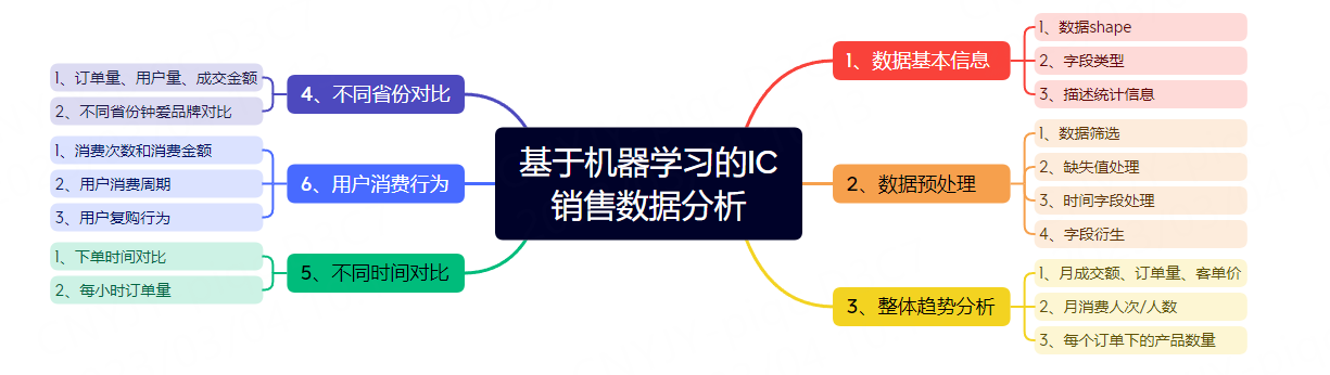
基于机器学习的IC电商数据挖掘-数据探索篇

基于机器学习的IC电子产品数据挖掘

最近获取到了一份IC电子产品电商数据的分析，后面会进行3个主题的数据分析：

1. 第一阶段：基于pandas、numpy、matplotlib、plotly等库的统计可视化分析
2. 第二阶段：基于机器学习聚类算法和RFM模型的用户画像分析
3. 第三阶段：基于关联规则算法的品牌、产品和产品种类关联性挖掘

本文是第一个阶段，主要内容包含：

• 数据预处理
• 数据探索EDA
• 多角度对比分析

导入库

In [1]:

import pandas as pd
import numpy as np

import time
import os
from datetime import datetime
import matplotlib.pyplot as plt
import seaborn as sns
%matplotlib inline
#设置中文编码和负号的正常显示
plt.rcParams['font.sans-serif']=['SimHei']
plt.rcParams['axes.unicode_minus']=False

import plotly_express as px
import plotly.graph_objects as go

import missingno as ms

from sklearn.cluster import KMeans
from sklearn.preprocessing import MinMaxScaler

数据基本信息

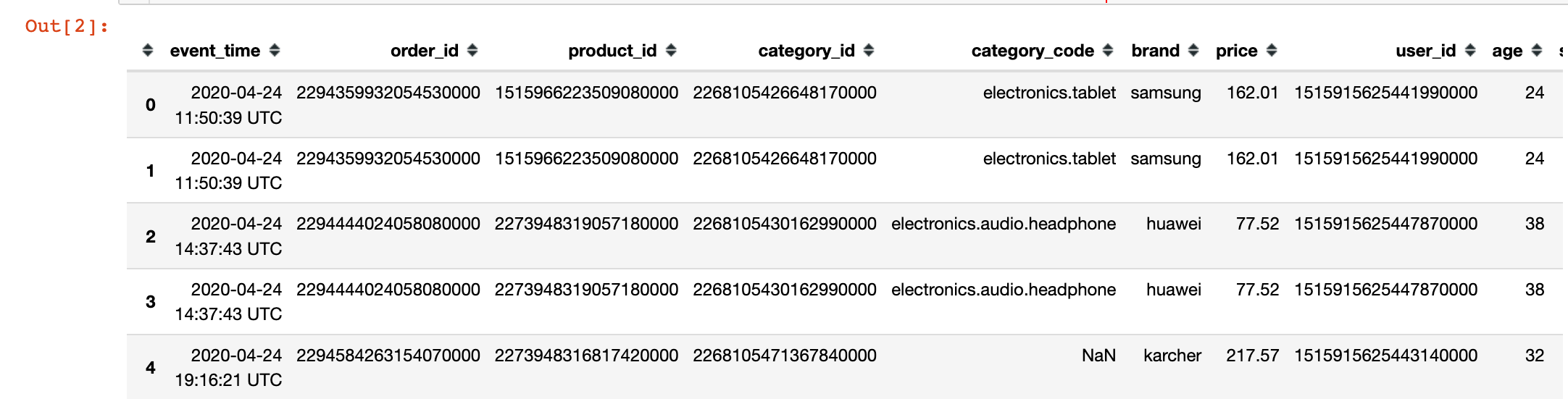
读取数据

df = pd.read_csv(
    "ic_sale.csv",
     encoding="utf-8",  # 指定编码
     converters={"order_id":str,"product_id":str,"category_id":str,"user_id":str} # 指定字段类型
)
df.head()

基本信息

In [3]:

# 1、数据shape

df.shape

Out[3]:

(564169, 11)

In [4]:

# 2、数据字段类型

df.dtypes

Out[4]:

event_time        object
order_id          object
product_id        object
category_id       object
category_code     object
brand             object
price            float64
user_id           object
age                int64
sex               object
local             object
dtype: object

In [5]:

# 3、数据描述统计信息

df.describe()

Out[5]:

	price	age
count	564169.000000	564169.000000
mean	208.269324	33.184388
std	304.559875	10.122088
min	0.000000	16.000000
25%	23.130000	24.000000
50%	87.940000	33.000000
75%	277.750000	42.000000
max	18328.680000	50.000000

In [6]:

# 4、总共多少个不同客户

df["user_id"].nunique()

Out[6]:

6908

In [7]:

# 5、总共多少个不同品牌

df["brand"].nunique()

Out[7]:

868

In [8]:

# 6、总共多少个订单

df["order_id"].nunique()

Out[8]:

234232

In [9]:

# 7、总共多少个产品

df["product_id"].nunique()

Out[9]:

3756

数据预处理

数据筛选

从描述统计信息中发现price字段的最小值是0，判定位异常；我们选择price大于0的信息：

In [10]:

df = df[df["price"] > 0]

缺失值处理

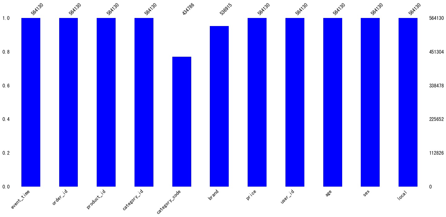
缺失值情况

In [11]:

df.isnull().sum()

Out[11]:

event_time            0
order_id              0
product_id            0
category_id           0
category_code    129344
brand             27215
price                 0
user_id               0
age                   0
sex                   0
local                 0
dtype: int64

可以看到缺失值体现在字段：

• category_code：类别
• brand：品牌

In [12]:

ms.bar(df,color="blue")  # 缺失值可视化

plt.show()

缺失值填充

In [13]:

df.fillna("missing",inplace=True)

In [14]:

df.isnull().sum()  # 填充之后无缺失值

Out[14]:

event_time       0
order_id         0
product_id       0
category_id      0
category_code    0
brand            0
price            0
user_id          0
age              0
sex              0
local            0
dtype: int64

时间字段处理

字段类型转化

读进来的数据中时间字段是object类型，需要将其转成时间格式的类型

In [15]:

df["event_time"][:5]   # 处理前

Out[15]:

0    2020-04-24 11:50:39 UTC
1    2020-04-24 11:50:39 UTC
2    2020-04-24 14:37:43 UTC
3    2020-04-24 14:37:43 UTC
4    2020-04-24 19:16:21 UTC
Name: event_time, dtype: object

In [16]:

# 去掉最后的UTC
df["event_time"] = df["event_time"].apply(lambda x: x[:19])

In [17]:

# 时间数据类型转化：字符类型---->指定时间格式

df['event_time'] = pd.to_datetime(df['event_time'], format="%Y-%m-%d %H:%M:%S")

字段衍生

In [18]:

# 提取多个时间相关字段

df['month']=df['event_time'].dt.month
df['day'] = df['event_time'].dt.day
df['dayofweek']=df['event_time'].dt.dayofweek
df['hour']=df['event_time'].dt.hour

In [19]:

df["event_time"][:5]   # 处理后

Out[19]:

0   2020-04-24 11:50:39
1   2020-04-24 11:50:39
2   2020-04-24 14:37:43
3   2020-04-24 14:37:43
4   2020-04-24 19:16:21
Name: event_time, dtype: datetime64[ns]

可以看到字段类型已经发生了变化

整体趋势分析

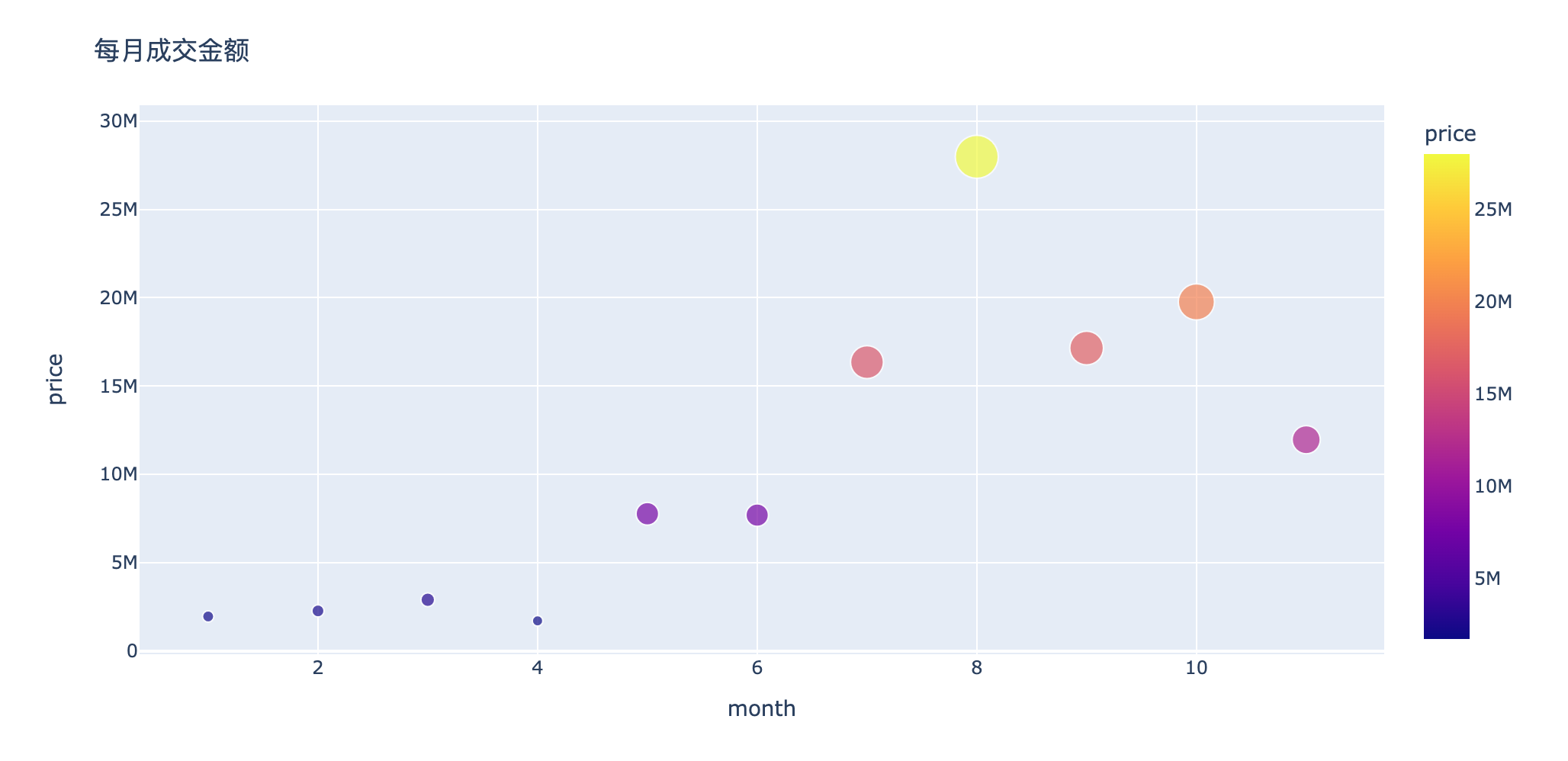
分析1：每月成交金额多少？

In [20]:

amount_by_month = df.groupby("month")["price"].sum().reset_index()
amount_by_month

Out[20]:

	month	price
0	1	1953358.17
1	2	2267809.88
2	3	2897486.26
3	4	1704422.41
4	5	7768637.79
5	6	7691244.33
6	7	16354029.27
7	8	27982605.44
8	9	17152310.57
9	10	19765680.76
10	11	11961511.52

In [21]:

fig = px.scatter(amount_by_month,x="month",y="price",size="price",color="price")

fig.update_layout(height=500, width=1000, title_text="每月成交金额")

fig.show()

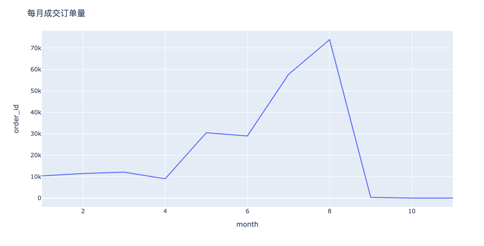
分析2：月订单量如何变化？

In [22]:

order_by_month = df.groupby("month")["order_id"].nunique().reset_index()
order_by_month

Out[22]:

	month	order_id
0	1	10353
1	2	11461
2	3	12080
3	4	9001
4	5	30460
5	6	28978
6	7	57659
7	8	73897
8	9	345
9	10	14
10	11	6

In [23]:

fig = px.line(order_by_month,x="month",y="order_id")

fig.update_layout(height=500, width=1000, title_text="每月成交订单量")

fig.show()

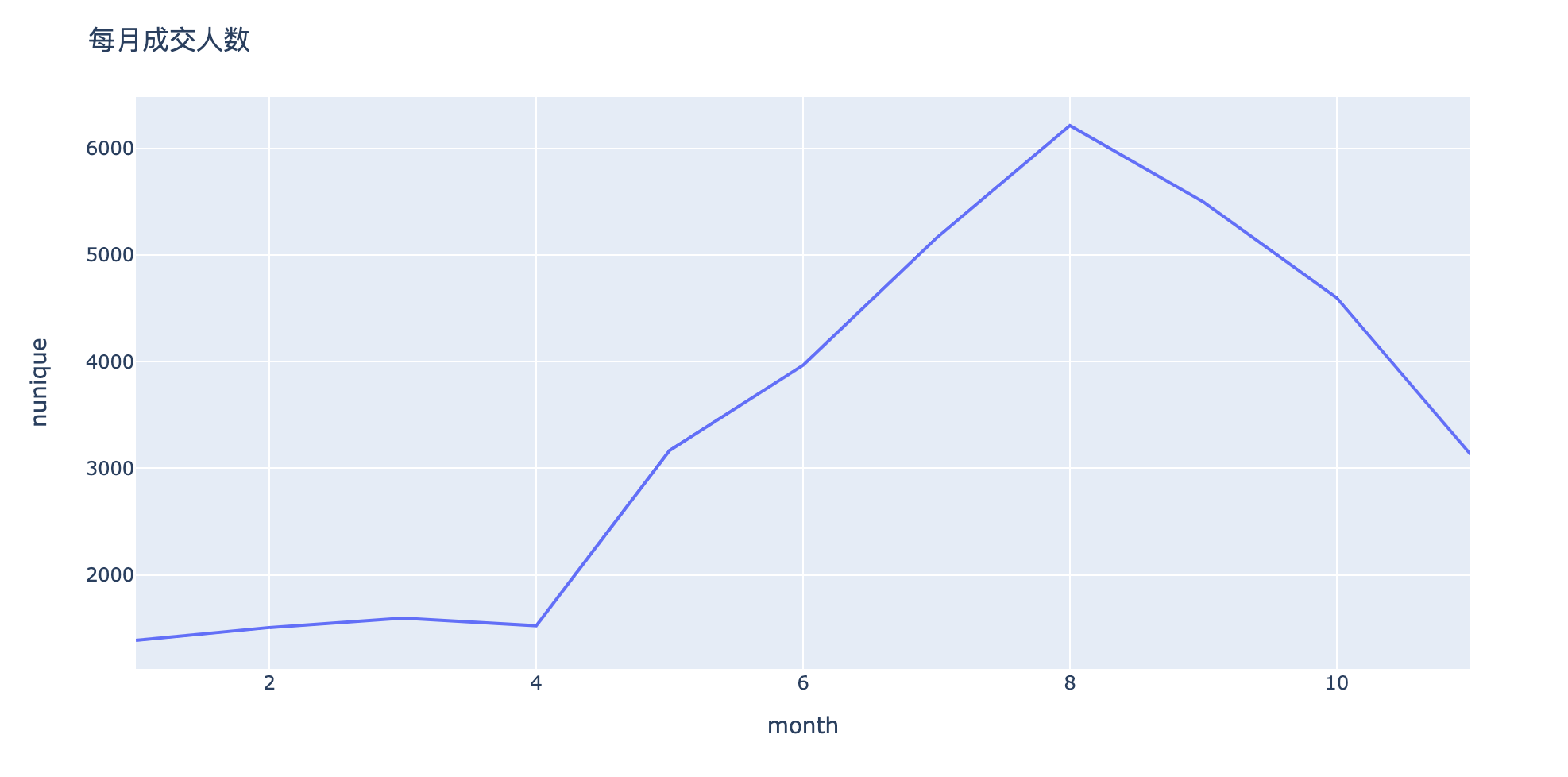
分析3：月消费人数/人次如何变化？

In [24]:

# nunique：对每个user_id进行去重：消费人数
# count：统计user_id 的次数；消费人次（存在一人多次购买）

people_by_month = df.groupby("month")["user_id"].agg(["nunique","count"]).reset_index()
people_by_month

Out[24]:

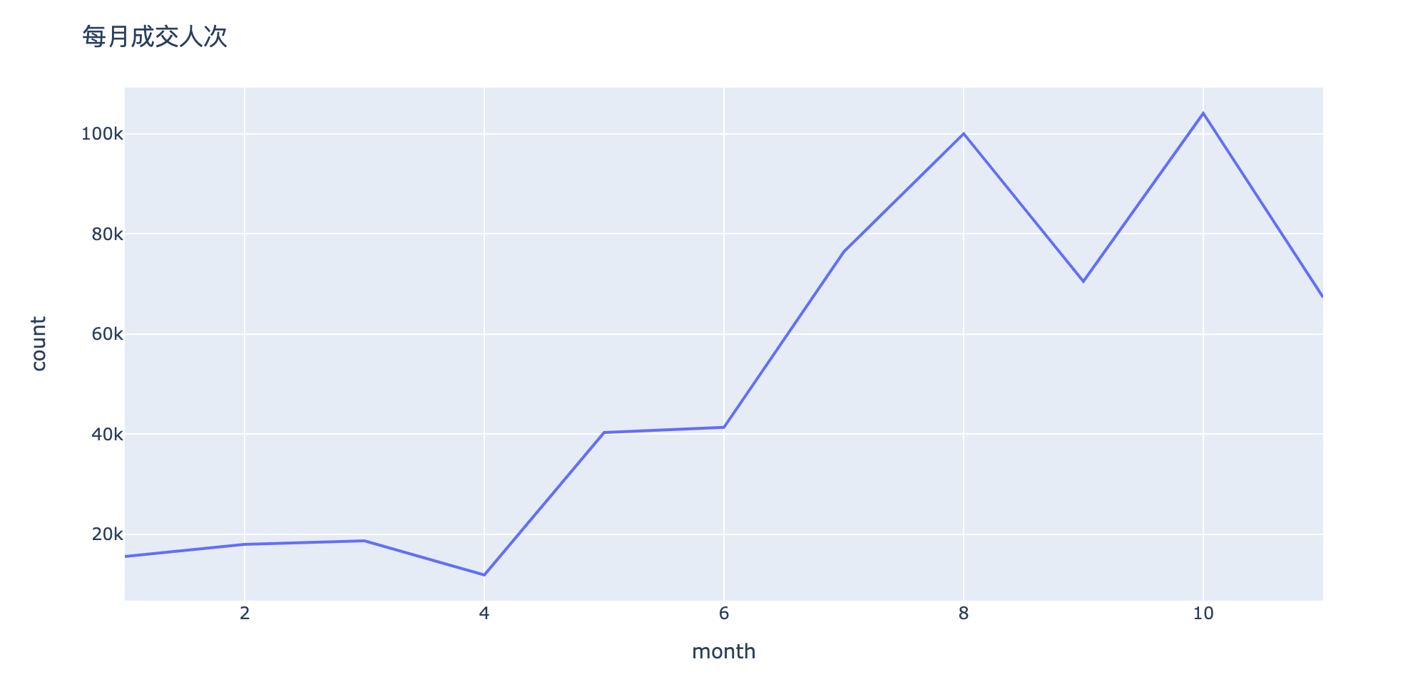
	month	nunique	count
0	1	1388	15575
1	2	1508	17990
2	3	1597	18687
3	4	1525	11867
4	5	3168	40332
5	6	3966	41355
6	7	5159	76415
7	8	6213	100006
8	9	5497	70496
9	10	4597	104075
10	11	3134	67332

In [25]:

fig = px.line(people_by_month,x="month",y="nunique")

fig.update_layout(height=500, width=1000, title_text="每月成交人数")

fig.show()

fig = px.line(people_by_month,x="month",y="count")

fig.update_layout(height=500, width=1000, title_text="每月成交人次")

fig.show()

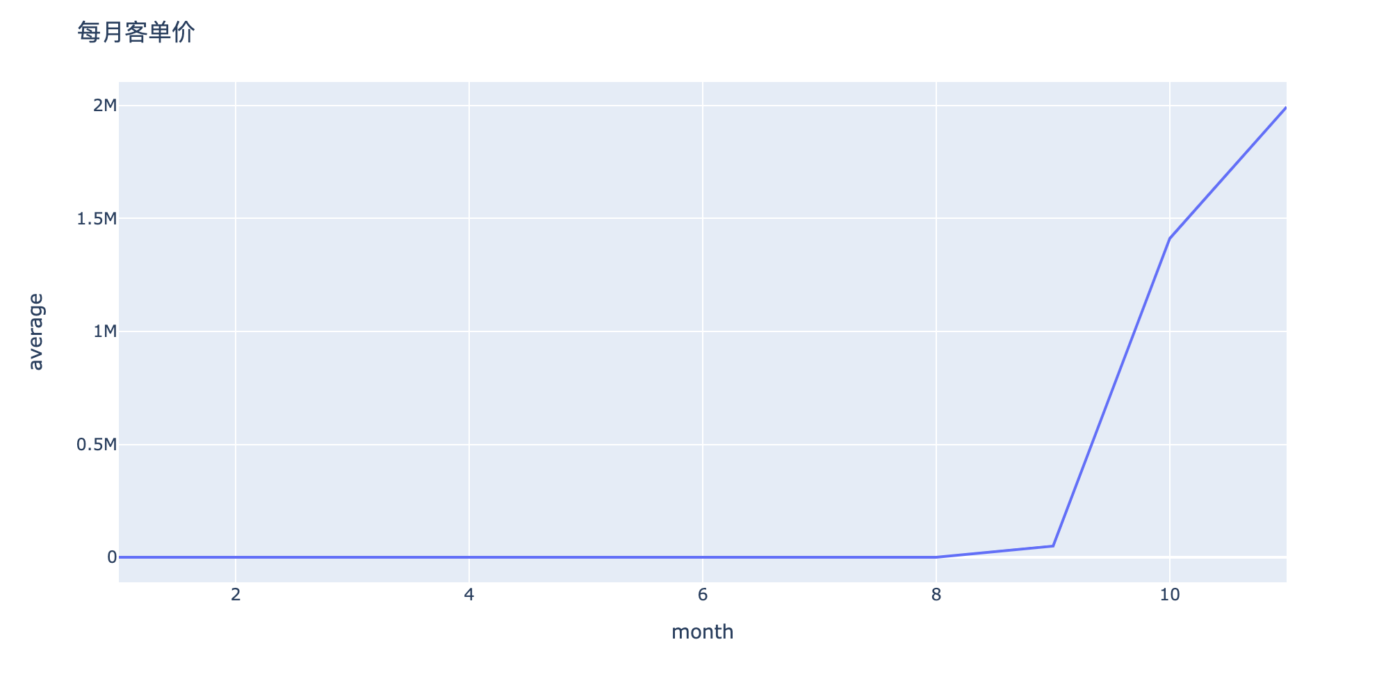
分析4：每月客单价多少？

In [27]:

amount_by_month  # 每月成交金额

Out[27]:

	month	price
0	1	1953358.17
1	2	2267809.88
2	3	2897486.26
3	4	1704422.41
4	5	7768637.79
5	6	7691244.33
6	7	16354029.27
7	8	27982605.44
8	9	17152310.57
9	10	19765680.76
10	11	11961511.52

In [28]:

order_by_month  # 每月订单数

Out[28]:

	month	order_id
0	1	10353
1	2	11461
2	3	12080
3	4	9001
4	5	30460
5	6	28978
6	7	57659
7	8	73897
8	9	345
9	10	14
10	11	6

In [29]:

amount_by_userid = pd.merge(amount_by_month,order_by_month)

amount_by_userid

Out[29]:

	month	price	order_id
0	1	1953358.17	10353
1	2	2267809.88	11461
2	3	2897486.26	12080
3	4	1704422.41	9001
4	5	7768637.79	30460
5	6	7691244.33	28978
6	7	16354029.27	57659
7	8	27982605.44	73897
8	9	17152310.57	345
9	10	19765680.76	14
10	11	11961511.52	6

In [30]:

amount_by_userid["average"] = amount_by_userid["price"] / amount_by_userid["order_id"]

amount_by_userid

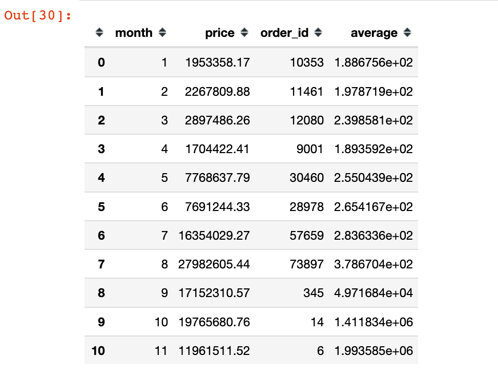
fig = px.line(amount_by_userid,x="month",y="average")

fig.update_layout(height=500, width=1000, title_text="每月客单价")

fig.show()

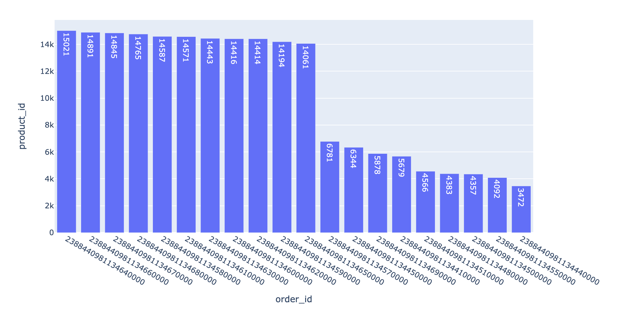
分析5：每个订单包含多少产品

In [32]:

product_by_order = df.groupby("order_id")["product_id"].count().reset_index().sort_values("product_id",ascending=False)

product_by_order.head(10)

Out[32]:

	order_id	product_id
234208	2388440981134640000	15021
234210	2388440981134660000	14891
234211	2388440981134670000	14845
234212	2388440981134680000	14765
234202	2388440981134580000	14587
234205	2388440981134610000	14571
234207	2388440981134630000	14443
234204	2388440981134600000	14416
234206	2388440981134620000	14414
234203	2388440981134590000	14194

In [33]:

fig = px.bar(product_by_order[:20],
             x="order_id",
             y="product_id",
             text="product_id"
            )

fig.show()

不同省份对比

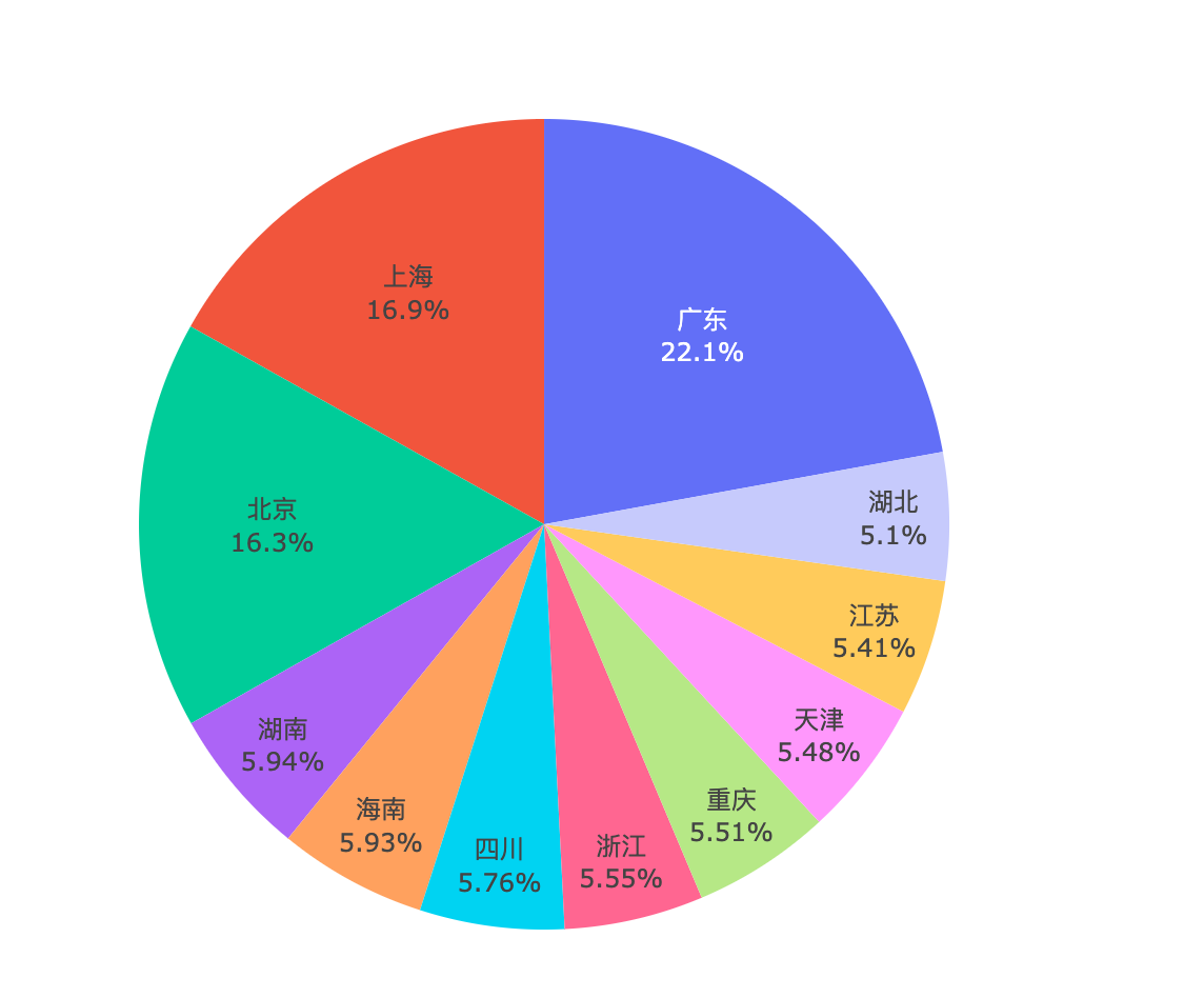
分析6：订单量、用户量和成交金额对比

不同省份下的订单量、用户量和成交金额对比

In [34]:

local = df.groupby("local").agg({"order_id":"nunique","user_id":"nunique","price":sum}).reset_index()
local.head()

Out[34]:

	local	order_id	user_id	price
0	上海	39354	5680	19837942.20
1	北京	38118	5702	19137748.75
2	四川	13396	3589	6770891.28
3	天津	13058	3497	6433736.85
4	广东	51471	6085	26013770.86

In [35]:

df1 = local.sort_values("order_id",ascending=True)  # 订单量升序
df1

Out[35]:

	local	order_id	user_id	price
6	浙江	12790	3485	6522657.59
8	湖北	12810	3488	5993820.57
3	天津	13058	3497	6433736.85
10	重庆	13058	3496	6479488.14
7	海南	13076	3587	6968674.41
2	四川	13396	3589	6770891.28
5	江苏	13575	3598	6357286.87
9	湖南	13879	3481	6983078.88
1	北京	38118	5702	19137748.75
0	上海	39354	5680	19837942.20
4	广东	51471	6085	26013770.86

In [36]:

fig = px.pie(df1, names="local",labels="local",values="price")

fig.update_traces(
    textposition="inside",
    textinfo="percent+label"
)

fig.show()

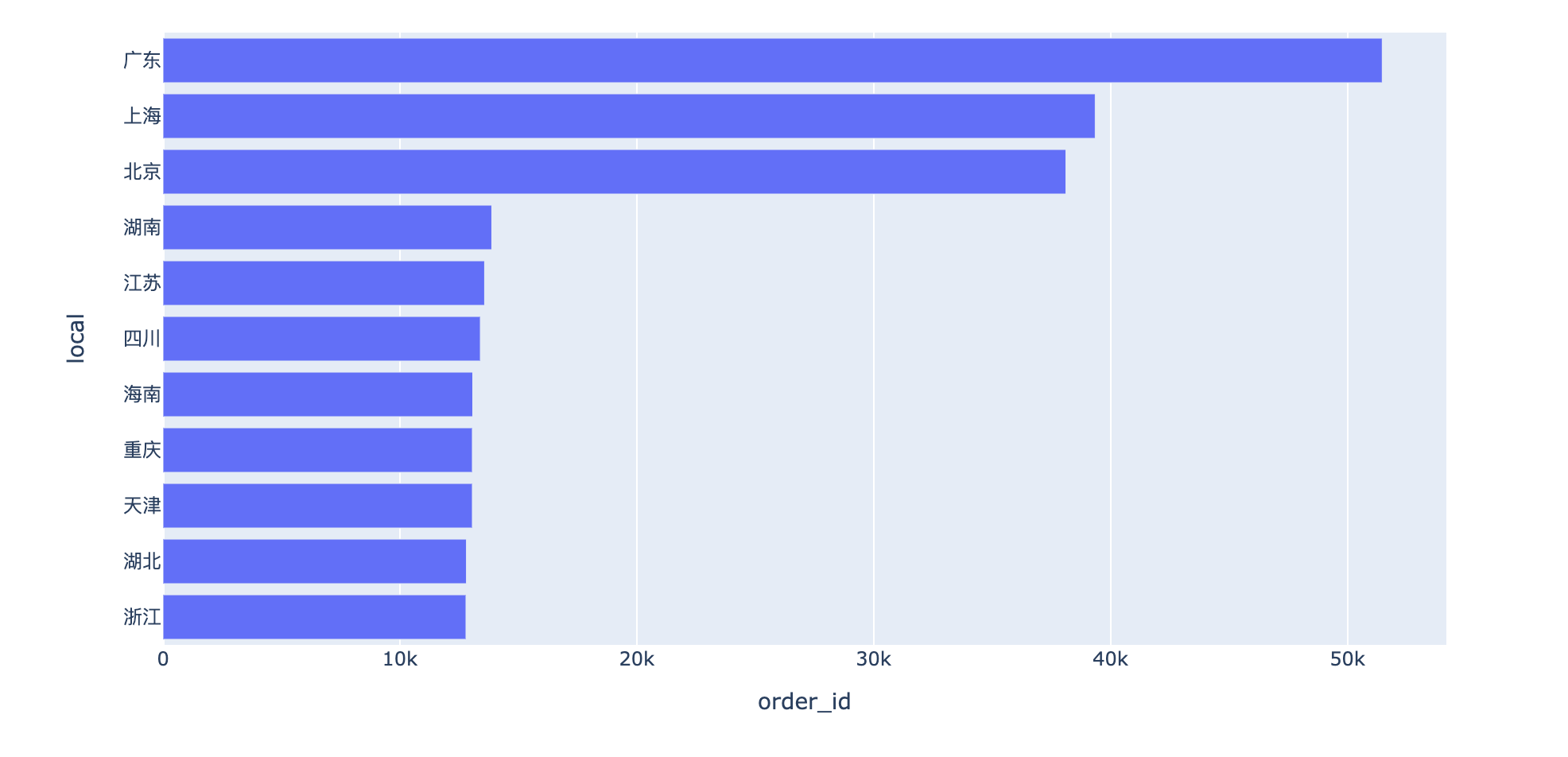
每个省份的订单量对比：

fig = px.bar(df1,x="order_id",y="local",orientation="h")

fig.show()

# 整体的可视化效果

fig = px.scatter_3d(local,
              x="order_id",
              y="user_id",
              z="price",
              color="order_id",
              hover_name="local"
             )

fig.show()

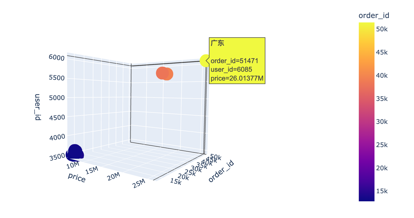
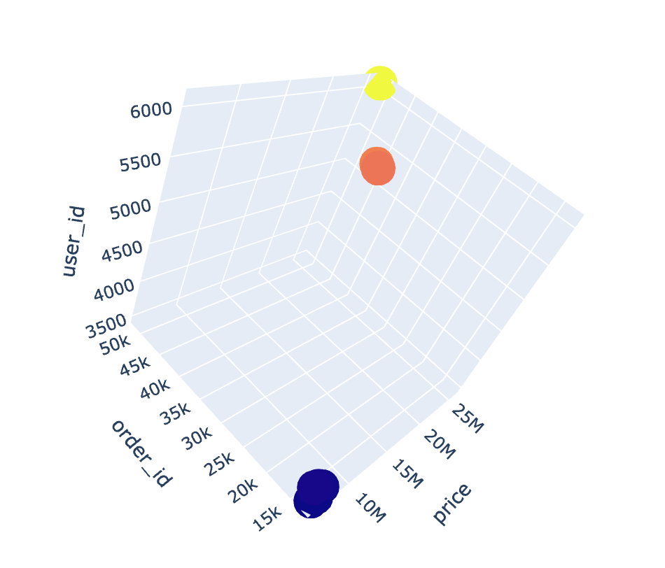
通过3D散点图我们发现：广东省真的是一骑绝尘！

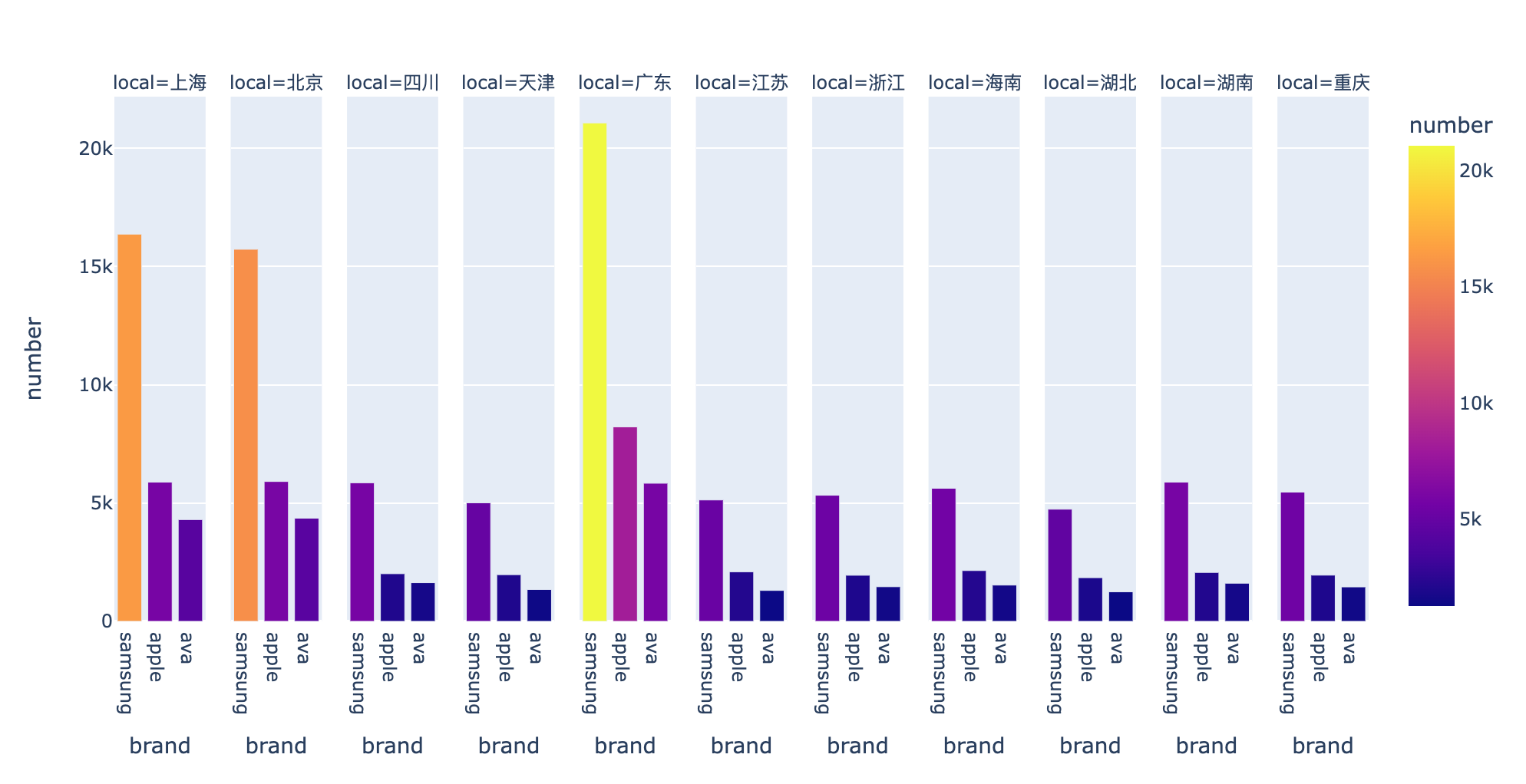
分析7：不同省份的客户钟爱哪些品牌？

In [39]:

local_brand = df.groupby(["local","brand"]).size().to_frame().reset_index()

local_brand.columns = ["local","brand","number"]  # 修改字段名

local_brand

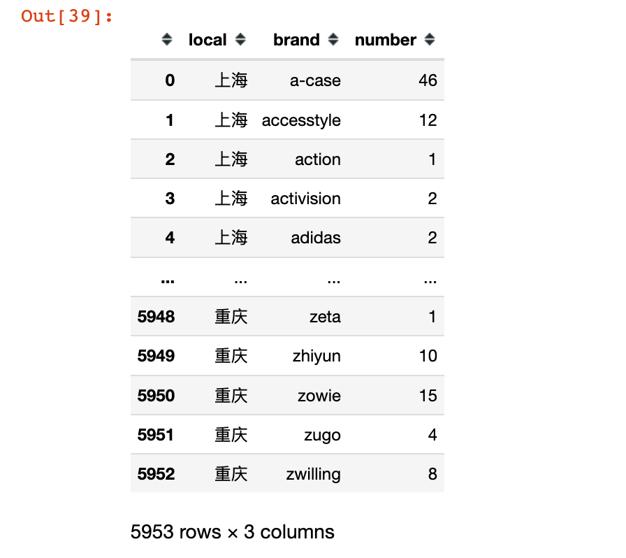
# 根据local和number进行排序
local_brand.sort_values(["local","number"],ascending=[True,False],inplace=True,ignore_index=True)
local_brand = local_brand[local_brand["brand"] != "missing"]
# 每个local下面最受欢迎的前3个品牌
local_brand = local_brand.groupby("local").head(3)
local_brand

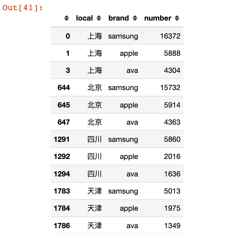
fig = px.bar(local_brand,
             x="brand",
             y="number",
             color="number",
             facet_col="local")

fig.update_layout(height=500,width=1000)

fig.show()

不同时间对比

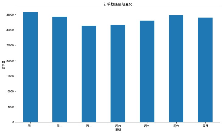
分析8：下单时间对比

In [43]:

df.columns

Out[43]:

Index(['event_time', 'order_id', 'product_id', 'category_id', 'category_code',
       'brand', 'price', 'user_id', 'age', 'sex', 'local', 'month', 'day',
       'dayofweek', 'hour'],
      dtype='object')

In [44]:

df2 = df.groupby("dayofweek")["order_id"].nunique().reset_index()
df2

Out[44]:

	dayofweek	order_id
0	0	35690
1	1	34256
2	2	31249
3	3	31555
4	4	33010
5	5	34772
6	6	33922

In [45]:

plt.figure(figsize=(12,7))

df2["order_id"].plot.bar()

plt.xticks(range(7),['周一','周二','周三','周四','周五','周六','周日'],rotation=0)
plt.xlabel('星期')
plt.ylabel('订单量')
plt.title('订单数随星期变化')

plt.show()

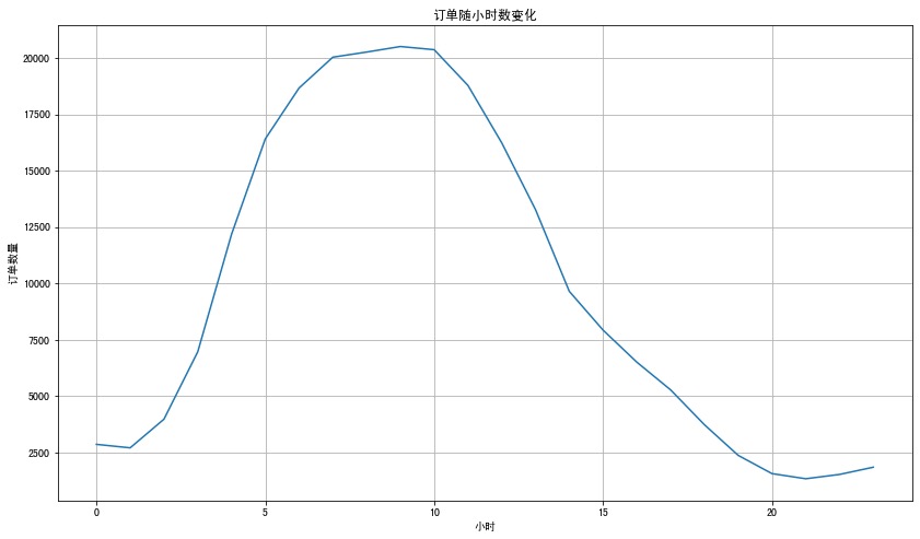
分析9：每小时订单量

In [46]:

df3 = df.groupby("hour")["order_id"].nunique().reset_index()
df3.head(10)

Out[46]:

	hour	order_id
0	0	2865
1	1	2711
2	2	3981
3	3	6968
4	4	12176
5	5	16411
6	6	18667
7	7	20034
8	8	20261
9	9	20507

In [47]:

plt.figure(figsize=(14,8))
df3["order_id"].plot()

plt.xlabel('小时')
plt.ylabel('订单数量')
plt.title('订单随小时数变化')

plt.grid()
plt.show()

不同用户消费行为分析

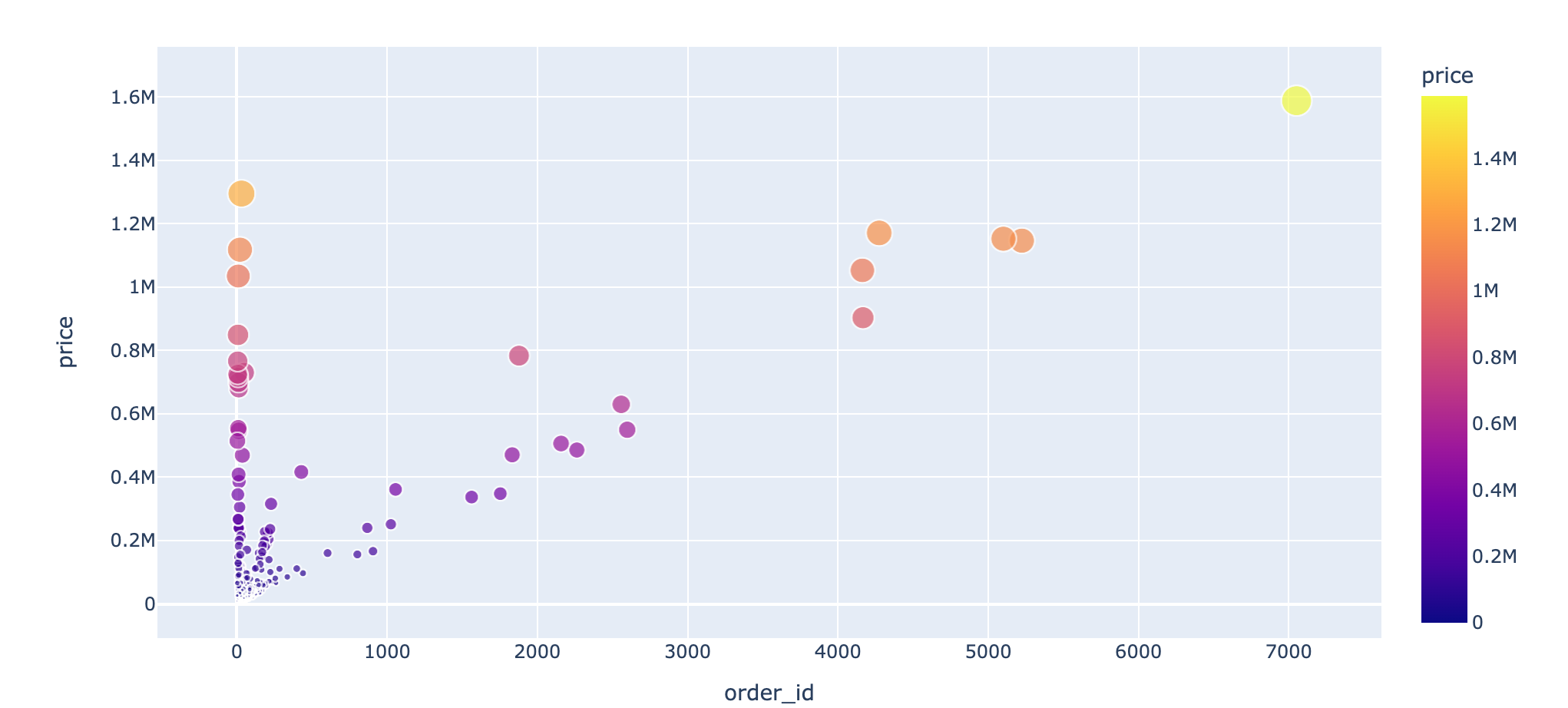
分析10：消费次数和消费金额

In [48]:

df4 = df.groupby("user_id").agg({"order_id":"nunique", "price":sum})

fig = px.scatter(df4,
                x="order_id",
                y="price",
                color="price",
                size="price")

fig.show()

分析11：用户消费周期

In [50]:

# 用户消费周期

# shift函数：移动一个单位

purchase_time=df.groupby('user_id').apply(lambda x: x['event_time'] - x['event_time'].shift()).dt.days
purchase_time

Out[50]:

user_id
1515915625439950000  96014      NaN
1515915625440030000  374760     NaN
                     484927    35.0
1515915625440050000  463812     NaN
                     473430     1.0
                               ...
1515915625514880000  564132     0.0
                     564143     0.0
                     564164     0.0
1515915625514890000  564158     NaN
                     564165     0.0
Name: event_time, Length: 564130, dtype: float64

In [51]:

purchase_time[purchase_time>0].describe()

Out[51]:

count    120629.000000
mean         35.494500
std         663.803583
min           1.000000
25%           2.000000
50%           4.000000
75%          12.000000
max       18466.000000
Name: event_time, dtype: float64

说明：

1. 至少消费两次的用户的消费周期是4天
2. 有75%的客户消费周期在12天

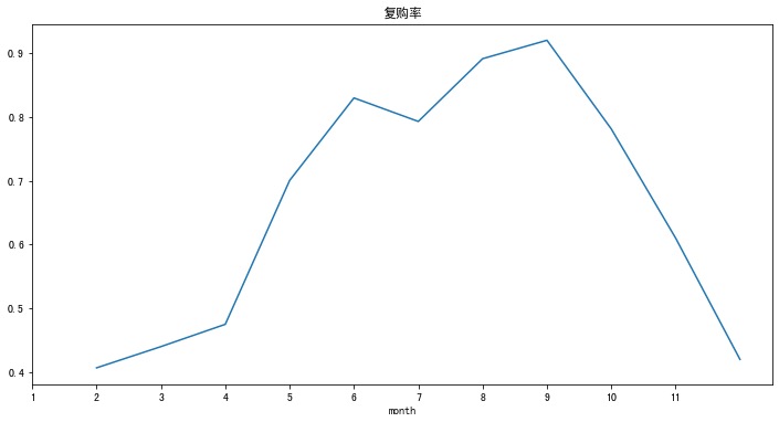
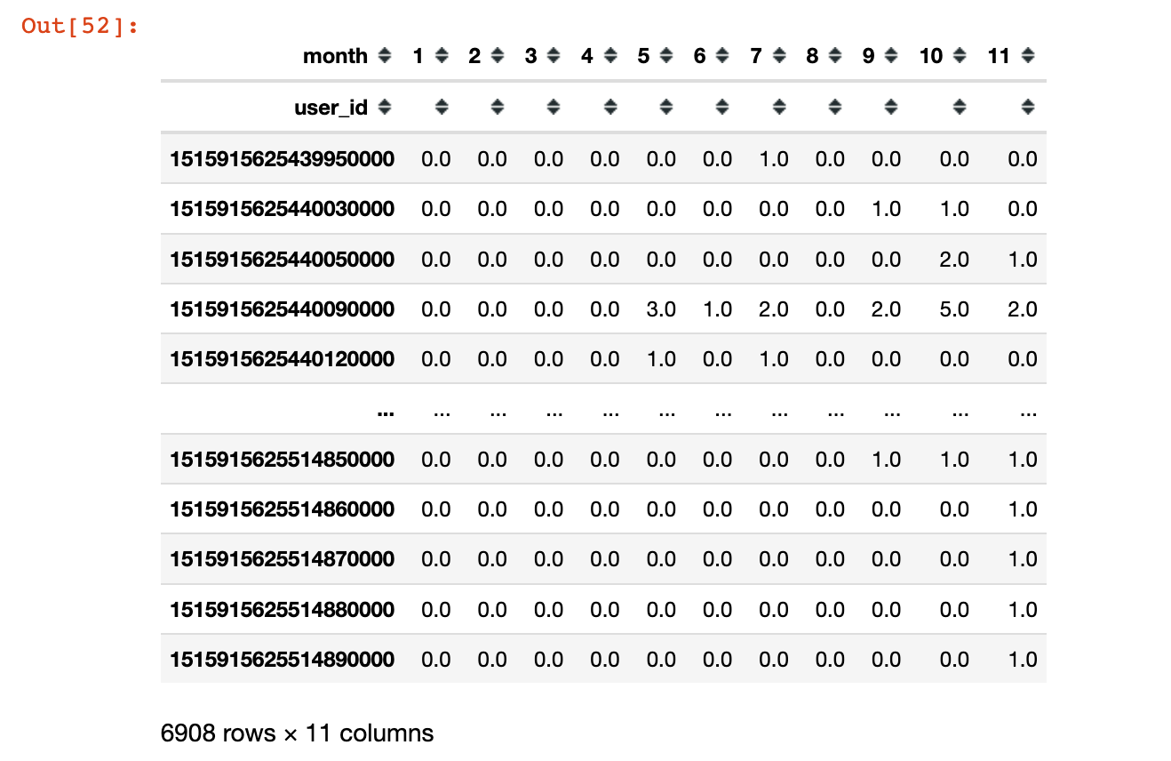
分析12：用户复购行为

In [52]:

pivoted_counts = df.pivot_table(index='user_id',
               columns='month',
               values='order_id',
               aggfunc='nunique').fillna(0)

pivoted_counts

Out[52]:

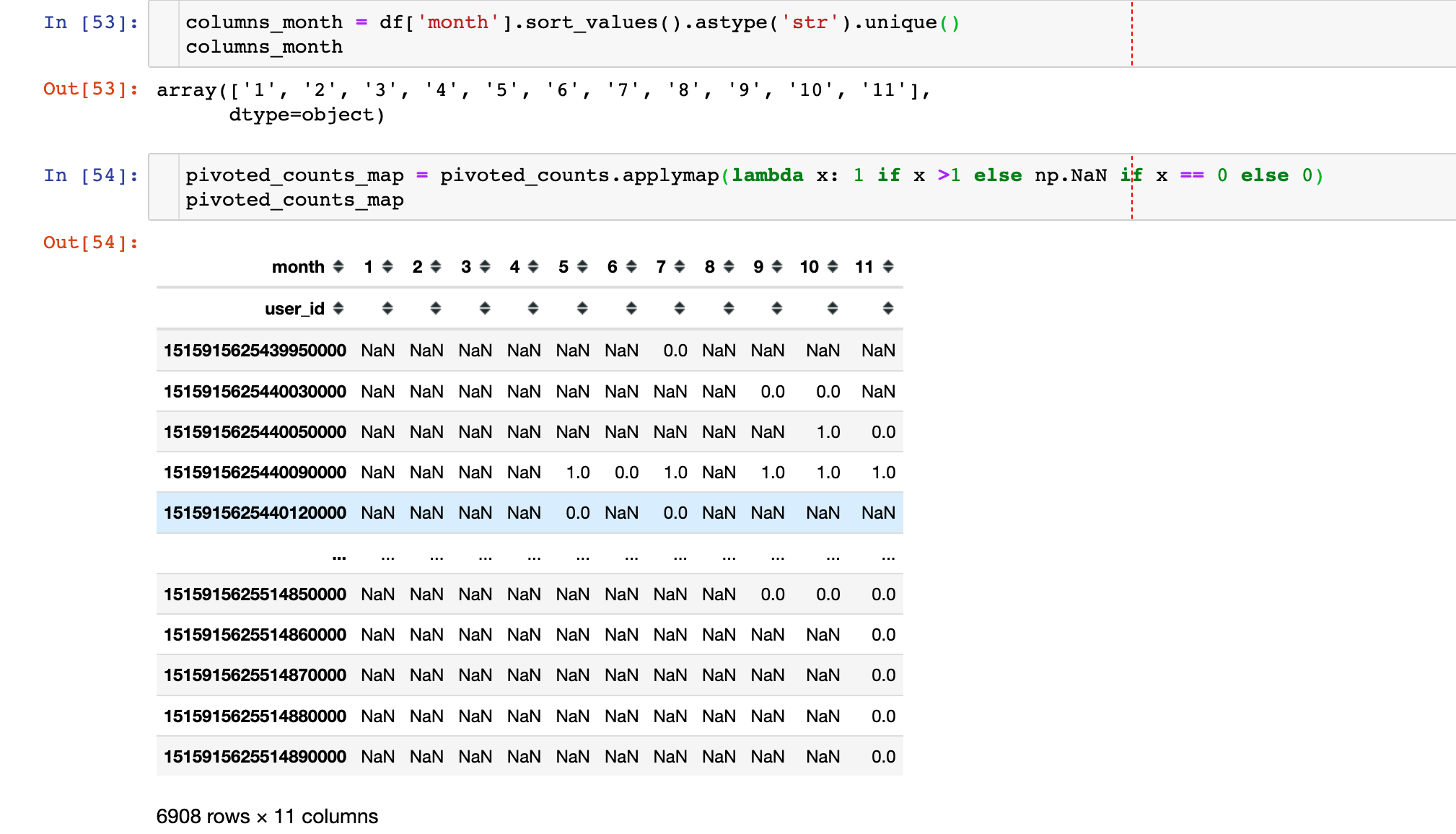
pivoted_counts_map.sum() / pivoted_counts_map.count()

# 结果
month
1     0.406340
2     0.439655
3     0.474640
4     0.700328
5     0.829861
6     0.792990
7     0.891452
8     0.920328
9     0.781153
10    0.609963
11    0.419592
dtype: float64

(pivoted_counts_map.sum()/pivoted_counts_map.count()).plot(figsize=(12,6))

plt.xticks(range(11),columns_month)

plt.title('复购率')
plt.show()