
对比计数统计和推理两种方法
本文记录的是书籍《深度学习进阶:自然语言处理》的第四章学习笔记。
基于计数的方法
基于计数的方法是根据一个单词周围的单词的出现次数来表示该单词。
- 生成单词的共现矩阵
- 进行降维SVD,获得密集向量
问题:语料库大的时候出现问题,维度爆炸和计算量增加。
基于推理的方法
使用神经网络的方法,通常在mini-batch数据上进行学习。
每次只需要学习部分数据;并且可以使用多台机器、多个GPU并行执行加速运算。
大致过程:
- 基于推理的方法引入某种模型(比如神经网络)
- 模型接收的上下文作为输入,输出各个单词的出现概率
- 模型产物:获得单词的分布式表示
神经网络中单词的处理方法
神经网络不能直接处理单词,需要将单词转化成固定长度的向量,使用one-hot编码:
- 出现单词的位置用1表示
- 没有出现对应单词的位置用0表示
向量内积np.dot实现
1 | import numpy as np |
array([[ 0.12477247, -0.25928347, -0.21568563]])
使用MatMul层实现
1 | class MatMul: |
1 | import sys |
array([[-0.23997344, -0.90521716, 0.74001086]])
简单的Word2Vec
使用由原版Word2Vec提出来的CBOW( continous bag-of-words)的模型作为神经网络。
两个经典的Word2Vec中使用的模型:
- CBOW模型
- skip-gram模型
CBOW模型推理
CBOW模型是根据上下文预测目标词的模型。
模型的输入:上下文,比如['you','goodbye']这样的单词,但是需要转化为one-hot编码表示。
本文中考虑上下文的两个单词,因此模型会有两个输入层。如果是考虑N个单词,则输入层有N个。
-
从输入层到中间层的变换使用相同的全连接层(权重都是$W_{in}$)
-
从中间层到输出层神经元的变换由另一个全连接层完成(权重是$W_{out}$)
中间层的神经元是各个输入层经全连接层变换后得到的值得平均。
输出层的神经元是各个单词的得分,它的值越大说明对应单词的出现概率值越高。
得分是指被解释为概率之前的值,对这些得分应用Softmax函数,就可以得到概率值。
代码实现
1 | import sys |
array([[-0.03647001,  1.22730525, -1.35937841,  1.0817182 ,  1.64785619,
         1.49898799, -0.18553477]])
CBOW模型的学习
CBOW模型的学习就是调整权重,以使其预测准确。
CBOW模型 + Softmax层 + Cross Entropy Error层
Word2Vec的权重和分布式表示
Word2Vec中使用的网络有两个权重,分别是输入侧的$W_{in}$和输出侧的$W_{out}$。
二者都是保存了单词含义进行了编码的向量,到底该选择哪个权重?最受欢迎的方案:只使用输入侧的权重
数据准备
上下文和目标词
- Word2Vec使用的神经网络的输入是上下文contexts;
- 它的正确标签是这些上下文包围在中间的单词,也就是目标词target。
使用语料库获取上下文和目标词
1 | # 第二章的precess函数 ;经常使用 |
1 | import sys |
array([0, 1, 2, 3, 4, 1, 5, 6])
1 | id_to_word |
{0: 'you', 1: 'say', 2: 'goodbye', 3: 'and', 4: 'i', 5: 'hello', 6: '.'}
1 | corpus[1:-1] |
array([1, 2, 3, 4, 1, 5])
1 | def create_contexts_target(corpus, window_size=1): |
1 | contexts, target = create_contexts_target(corpus, window_size=1) |
1 | contexts # 上下文 |
array([[0, 2],
       [1, 3],
       [2, 4],
       [3, 1],
       [4, 5],
       [1, 6]])
1 | target # 目标值 |
array([1, 2, 3, 4, 1, 5])
convert_one_hot:转成one-hot编码
1 | def convert_one_hot(corpus, vocab_size): |
1 | #text = 'You say goodbye and I say hello.' |
1 | target # 转成One-Hot编码后的形式 |
array([[0, 1, 0, 0, 0, 0, 0],
       [0, 0, 1, 0, 0, 0, 0],
       [0, 0, 0, 1, 0, 0, 0],
       [0, 0, 0, 0, 1, 0, 0],
       [0, 1, 0, 0, 0, 0, 0],
       [0, 0, 0, 0, 0, 1, 0]])
1 | contexts # 转成One-Hot编码后的形式 |
array([[[1, 0, 0, 0, 0, 0, 0],
        [0, 0, 1, 0, 0, 0, 0]],

       [[0, 1, 0, 0, 0, 0, 0],
        [0, 0, 0, 1, 0, 0, 0]],

       [[0, 0, 1, 0, 0, 0, 0],
        [0, 0, 0, 0, 1, 0, 0]],

       [[0, 0, 0, 1, 0, 0, 0],
        [0, 1, 0, 0, 0, 0, 0]],

       [[0, 0, 0, 0, 1, 0, 0],
        [0, 0, 0, 0, 0, 1, 0]],

       [[0, 1, 0, 0, 0, 0, 0],
        [0, 0, 0, 0, 0, 0, 1]]])
简单CBOW模型实现
交叉损失熵Crossentropy-Error
1 | def cross_entropy_error(y, t): |
SoftmaxWithLoss层实现
1 | # 定义softmax函数 |
SimpleCBOW类实现
1 | import sys |
基于上下文的正向传播forward
1 | # def forward(self, contexts, target): |
CBOW模型的反向传播
1 | # def backward(self, dout=1): |
Trainer类实现
1 | # 参数去重 |
SGD优化
1 | class SGD: |
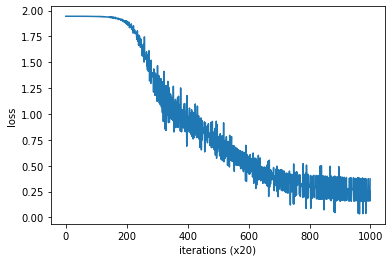
案例实战
1 | window_size = 1 |
词向量权重和ID分布式表示
1 | word_vecs = model.word_vecs # 变量权重 |
you [ 0.56529504 -0.89804494  2.2253568  -0.06463418 -1.1290963 ]
say [-1.1766486   0.99819845 -1.1207973   0.6008937   1.1576382 ]
goodbye [ 1.5599341   0.2788804  -0.38262236 -0.35986307 -1.1309035 ]
and [-0.8373688  -0.9373508  -1.2509673   1.8487976   0.51270753]
i [ 1.593292   0.2917557 -0.3518384 -0.3507546 -1.129358 ]
hello [ 0.5445614  -0.89658004  2.2065814  -0.07632335 -1.112859  ]
. [-0.3468702   1.9544731   0.13033707 -1.2471999   0.658087  ]
将单词表示为了密集向量,这就是单词的分布式表示
