kaggle绝技-离群点定位与处理

kaggle离群点分析

本文是针对kaggle上面一份关于数据离群点的分析，主要是介绍如何从数据中快速确定离群点outlier

原文地址：https://www.kaggle.com/code/nareshbhat/outlier-the-silent-killer

原文标题：Outlier!!! The Silent Killer

什么是离群点

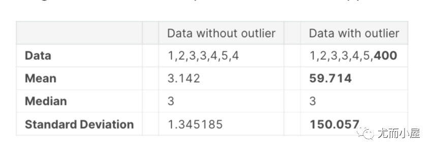
Outlier is an observation that is numerically distant from the rest of the data or in a simple word it is the value which is out of the range.let’s take an example to check what happens to a data set with and data set without outliers.

简答地说：离群值就是和正常值相差甚远的值。

看一个例子：在下面例子的数据中400就是一个离群点。

Outlier is a commonly used terminology by analysts and data scientists as it needs close attention else it can result in wildly wrong estimations. Simply speaking, Outlier is an observation that appears far away and diverges from an overall pattern in a sample.

离群值是分析师和数据科学家常用术语，因为它需要密切关注，否则可能会导致严重错误的估计。简单来说，离群值是一种观察结果，它看起来很远并且偏离了样本中的整体模式。

离群值如何产生？

• Data Entry Errors:- Human errors such as errors caused during data collection, recording, or entry can cause outliers in data.
• Measurement Error:- It is the most common source of outliers. This is caused when the measurement instrument used turns out to be faulty.
• Natural Outlier:- When an outlier is not artificial (due to error), it is a natural outlier. Most of real world data belong to this category.

1. 数据输入错误：- 人为错误，例如在数据收集、记录或输入过程中造成的错误，可能会导致数据出现异常值。
2. 测量误差：- 这是异常值的最常见来源。这是由于使用的测量仪器出现故障造成的。
3. 自然异常值：- 当异常值不是人为的（由于错误）时，它就是自然异常值。大多数现实世界的数据都属于这一类。

离群点类型

有两种类型：基于单变量和多变量的类型。上面的例子就是基于单变量，当我们查看单个变量的分布时，可以找到这些异常值。多变量异常值是 n 维空间中的异常值。

确定离群点方法

1. Hypothesis Testing - 假设检验
2. Z-score method-Z-score法
3. Robust Z-score-稳健Z分数
4. I.Q.R method-I.Q.R方法
5. Winsorization method(Percentile Capping)-Winsorization方法
6. DBSCAN Clustering-DBSCAN聚类
7. Isolation Forest-孤立森林
8. Visualizing the data-可视化数据

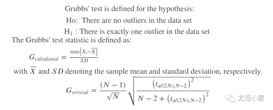
假设检验-格鲁布斯检验方法

基于格鲁布斯检验法：

资料1：https://zhuanlan.zhihu.com/p/482006257

资料2：https://blog.csdn.net/sunshihua12829/article/details/49047087

# 忽略警告
import warnings
warnings.filterwarnings("ignore")

import numpy as np
import scipy.stats as stats
x = np.array([12,13,14,19,21,23])
y = np.array([12,13,14,19,21,23,45])

def grubbs_test(x):
    n = len(x)
    mean_x = np.mean(x)  # 均值
    sd_x = np.std(x)  # 标准差
    numerator = max(abs(x-mean_x))  # 最大绝对误差
    g_calculated = numerator/sd_x  # 计算格鲁布斯值
    print("Grubbs Calculated Value:",g_calculated)
    t_value = stats.t.ppf(1 - 0.05 / (2 * n), n - 2)
    g_critical = ((n - 1) * np.sqrt(np.square(t_value))) / (np.sqrt(n) * np.sqrt(n - 2 + np.square(t_value)))
    print("Grubbs Critical Value:",g_critical)
    if g_critical > g_calculated:
        print("无离群点")
    else:
        print("存在离群点")

grubbs_test(x)
grubbs_test(y)

Grubbs Calculated Value: 1.4274928542926593
Grubbs Critical Value: 1.887145117792422
无离群点
Grubbs Calculated Value: 2.2765147221587774
Grubbs Critical Value: 2.019968507680656
存在离群点

Z-SCORE METHOD

参考1：https://zhuanlan.zhihu.com/p/69074703

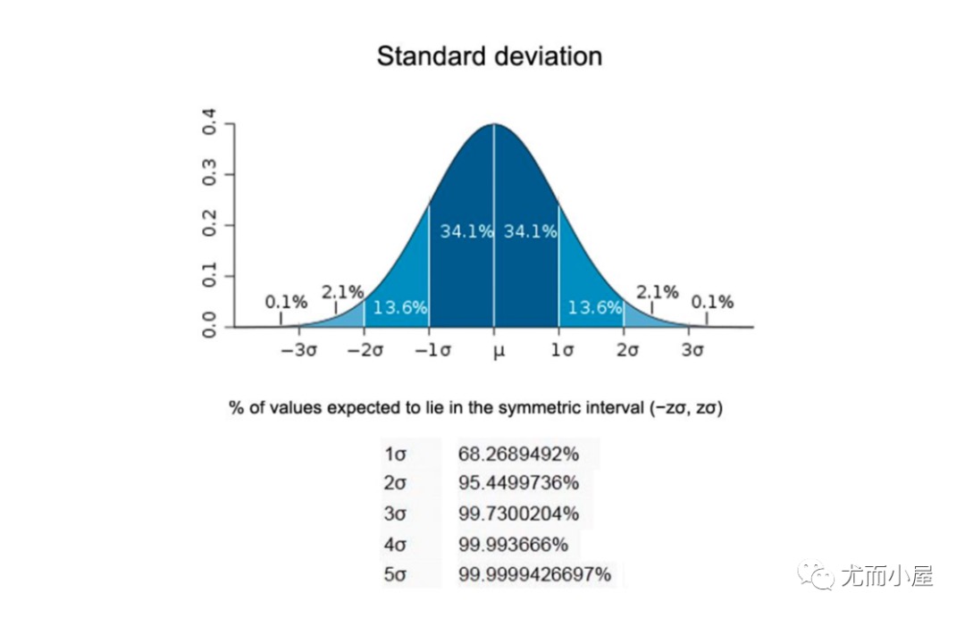
Z-score值的计算：

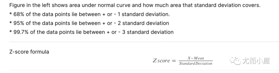
$$Z_{score} = \frac{X-Mean} {StandarDeviation}$$

import pandas as pd
import numpy as np

# 使用的数据df
train = pd.read_csv('House.csv')

out=[]

def Zscore_outlier(df):
    m = np.mean(df)  # 均值
    sd = np.std(df)  # 标准差
    for i in df:
        z = (i-m)/sd
        if np.abs(z) > 3:
            out.append(i)
    print("Outliers:",out)
Zscore_outlier(train['LotArea'])

Outliers: [50271, 159000, 215245, 164660, 53107, 70761, 53227, 46589, 115149, 53504, 45600, 63887, 57200]

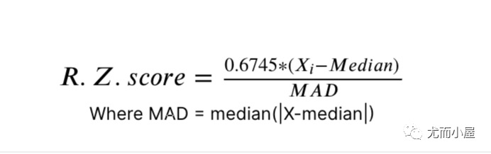
ROBUST Z-SCORE

It is also called as Median absolute deviation method. It is similar to Z-score method with some changes in parameters. Since mean and standard deviations are heavily influenced by outliers, alter to this parameters we use median and absolute deviation from median.

它也被称为中值绝对偏差法。它类似于 Z-score 方法，只是参数有所变化。由于均值和标准差受异常值的影响很大，因此我们使用中位数和中位数的绝对偏差来更改此参数。

import pandas as pd
import numpy as np
train = pd.read_csv('House.csv')

out=[]
def ZRscore_outlier(df):
    med = np.median(df)
    ma = stats.median_absolute_deviation(df)
    for i in df:
        z = (0.6745*(i-med))/ (np.median(ma))
        if np.abs(z) > 3:
            out.append(i)
    print("Outliers:",out)
ZRscore_outlier(train['LotArea'])

Outliers: [50271, 31770, 22950, 25419, 159000, 39104, 215245, 164660, 53107, 34650, 70761, 53227, 40094, 32668, 25095, 46589, 26178, 115149, 53504, 28698, 45600, 25286, 27650, 24090, 25000, 29959, 23257, 35760, 35133, 32463, 24682, 23595, 36500, 63887, 25339, 57200, 26142]

IQR METHOD

在这种使用四分位数间距 (IQR) 的方法中，我们检测异常值。 IQR 告诉我们数据集中的变化。任何超出 -1.5 x IQR 到 1.5 x IQR 范围的值都被视为异常值。

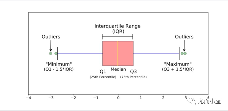
• Q1 表示数据的第一个四分位数/第 25 个百分位数。
• Q2 表示数据的第二个四分位数/中位数/第 50 个百分位数。
• Q3 表示数据的第 3 个四分位数/第 75 个百分位数。
• (Q1–1.5IQR) 代表数据集中的最小值，(Q3+1.5IQR) 代表数据集中的最大值。

import pandas as pd
import numpy as np
train = pd.read_csv('House.csv')

out=[]
def iqr_outliers(df):
    q1 = df.quantile(0.25)
    q3 = df.quantile(0.75)
    iqr = q3-q1
    Lower_tail = q1 - 1.5 * iqr
    Upper_tail = q3 + 1.5 * iqr
    for i in df:
        if i > Upper_tail or i < Lower_tail:
            out.append(i)
    print("Outliers:",out)
iqr_outliers(train['LotArea'])

Outliers: [50271, 19900, 21000, 21453, 19378, 31770, 22950, 25419, 159000, 19296, 39104, 19138, 18386, 215245, 164660, 20431, 18800, 53107, 34650, 22420, 21750, 70761, 53227, 40094, 32668, 21872, 21780, 25095, 46589, 20896, 18450, 21535, 26178, 115149, 21695, 53504, 21384, 28698, 45600, 17920, 25286, 27650, 24090, 25000, 1300, 21286, 1477, 21750, 29959, 18000, 23257, 17755, 35760, 18030, 35133, 32463, 18890, 24682, 23595, 17871, 36500, 63887, 20781, 25339, 57200, 20544, 19690, 21930, 26142]

缩尾处理-WINSORIZATION METHOD(PERCENTILE CAPPING)

这种方法类似于 IQR 方法。如果一个值超过第 99 个百分位数的值并且低于给定值的第一个百分位数，则将被视为异常值。

import pandas as pd
import numpy as np
train = pd.read_csv('Titanic.csv')
out=[]

def Winsorization_outliers(df):
    q1 = np.percentile(df , 1)
    q3 = np.percentile(df , 99)
    for i in df:
        if i > q3 or i < q1:
            out.append(i)
    print("Outliers:",out)
Winsorization_outliers(train['Fare'])

Outliers: [263.0, 263.0, 512.3292, 262.375, 263.0, 263.0, 512.3292, 512.3292, 262.375]

聚类-DBSCAN（基于密度的应用噪声空间聚类）

DBSCAN 是一种基于密度的聚类算法，它将数据集划分为高密度区域的子组，并将高密度区域聚类识别为异常值

import pandas as pd
from sklearn.cluster import DBSCAN
train = pd.read_csv('Titanic.csv')

def DB_outliers(df):
    outlier_detection = DBSCAN(eps = 2, metric='euclidean', min_samples = 5)
    clusters = outlier_detection.fit_predict(df.values.reshape(-1,1))
    data = pd.DataFrame()
    data['cluster'] = clusters
    print(data['cluster'].value_counts().sort_values(ascending=False))
DB_outliers(train['Fare'])

 0     705
 2      50
 4      36
-1      32
 6      15
 1      12
 7       8
 5       7
 8       7
 9       7
 3       6
 10      6
Name: cluster, dtype: int64

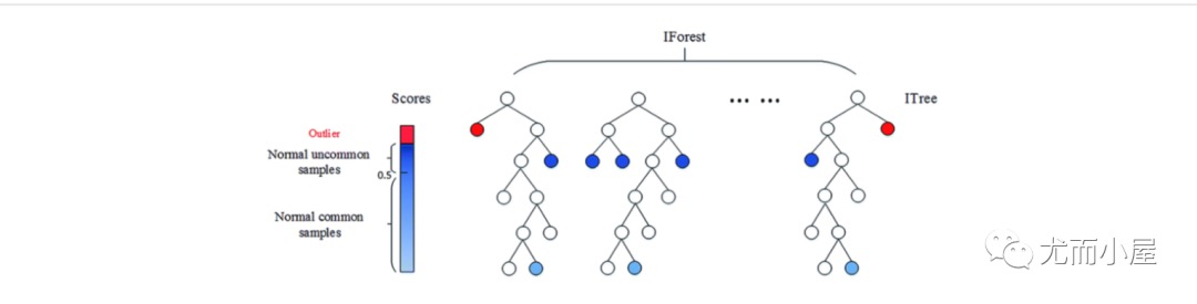
孤立森林-ISOLATION FOREST

它是一种属于集成决策树家族的聚类算法，在原理上类似于随机森林

from sklearn.ensemble import IsolationForest
import numpy as np
import pandas as pd
train = pd.read_csv('Titanic.csv')
train['Fare'].fillna(train[train.Pclass==3]['Fare'].median(),inplace=True)


def Iso_outliers(df):
    iso = IsolationForest(random_state = 1, contamination= 'auto')
    preds = iso.fit_predict(df.values.reshape(-1,1))
    data = pd.DataFrame()
    data['cluster'] = preds
    print(data['cluster'].value_counts().sort_values(ascending=False))
Iso_outliers(train['Fare'])

 1    706
-1    185
Name: cluster, dtype: int64

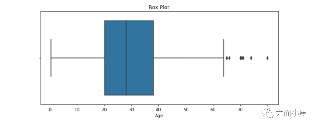
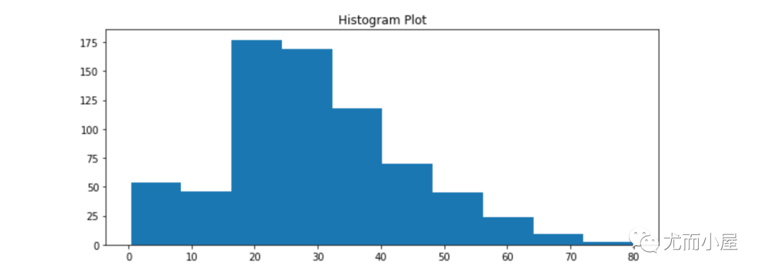
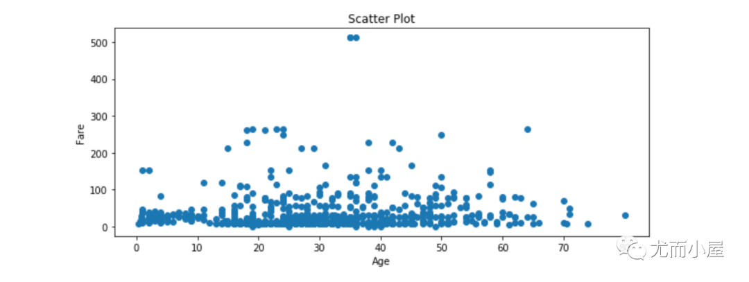
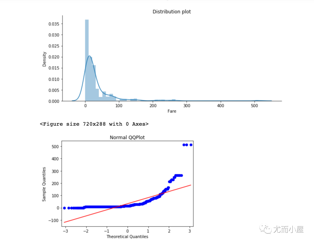
基于数据可视化

通过箱型图、散点图、直方图、两两分布图、QQ图等将数据进行可视化，通过观察来找到离群点

import pandas as pd
import seaborn as sns
from matplotlib import pyplot as plt
from statsmodels.graphics.gofplots import qqplot
train = pd.read_csv('Titanic.csv')

def Box_plots(df):
    plt.figure(figsize=(10, 4))
    plt.title("Box Plot")
    sns.boxplot(df)
    plt.show()

Box_plots(train['Age'])

def hist_plots(df):
    plt.figure(figsize=(10, 4))
    plt.hist(df)
    plt.title("Histogram Plot")
    plt.show()
hist_plots(train['Age'])

def scatter_plots(df1,df2):
    fig, ax = plt.subplots(figsize=(10,4))
    ax.scatter(df1,df2)
    ax.set_xlabel('Age')
    ax.set_ylabel('Fare')
    plt.title("Scatter Plot")
    plt.show()
scatter_plots(train['Age'],train['Fare'])

def dist_plots(df):
    plt.figure(figsize=(10, 4))
    sns.distplot(df)
    plt.title("Distribution plot")
    sns.despine()
    plt.show()
dist_plots(train['Fare'])

def qq_plots(df):
    plt.figure(figsize=(10, 4))
    qqplot(df,line='s')
    plt.title("Normal QQPlot")
    plt.show()
qq_plots(train['Fare'])

异常值处理

上面介绍的内容是如何发现数据中的离群点。在找到离群点后，如何处理？

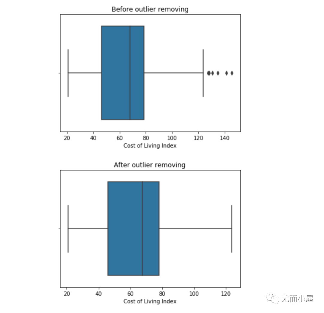
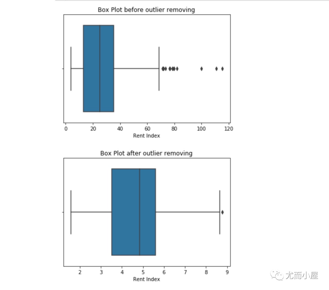
处理1：删除离群点

import pandas as pd
import numpy as np
import seaborn as sns
from matplotlib import pyplot as plt
train = pd.read_csv('cost-of-living-2018.csv')
sns.boxplot(train['Cost of Living Index'])
plt.title("Before outlier removing")
plt.show()  # 删除前


# 基于IQR方法删除离群点
def drop_outliers(df, field_name):
    iqr = 1.5 * (np.percentile(df[field_name], 75) - np.percentile(df[field_name], 25))
    df.drop(df[df[field_name] > (iqr + np.percentile(df[field_name], 75))].index, inplace=True)
    df.drop(df[df[field_name] < (np.percentile(df[field_name], 25) - iqr)].index, inplace=True)
drop_outliers(train, 'Cost of Living Index')
sns.boxplot(train['Cost of Living Index'])
plt.title("After outlier removing")
plt.show()   # 删除后

处理2：数据转换

介绍4种数据转换的方法：

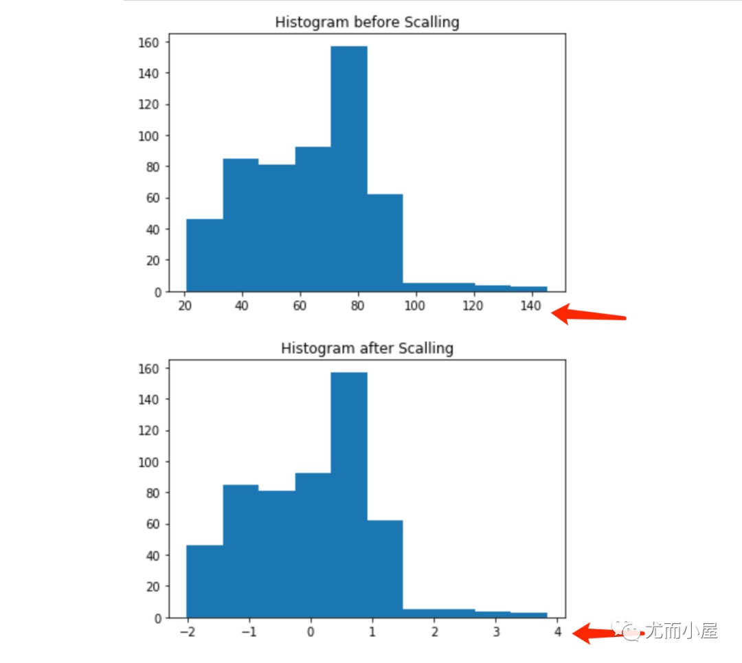
1. 尺度缩放：Scalling
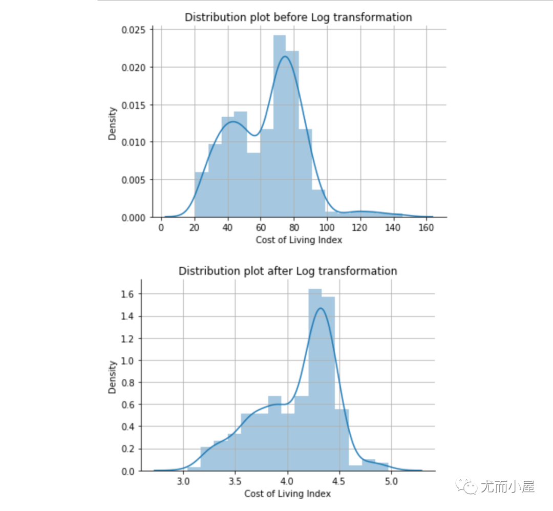
2. 对数变换：Log transformation
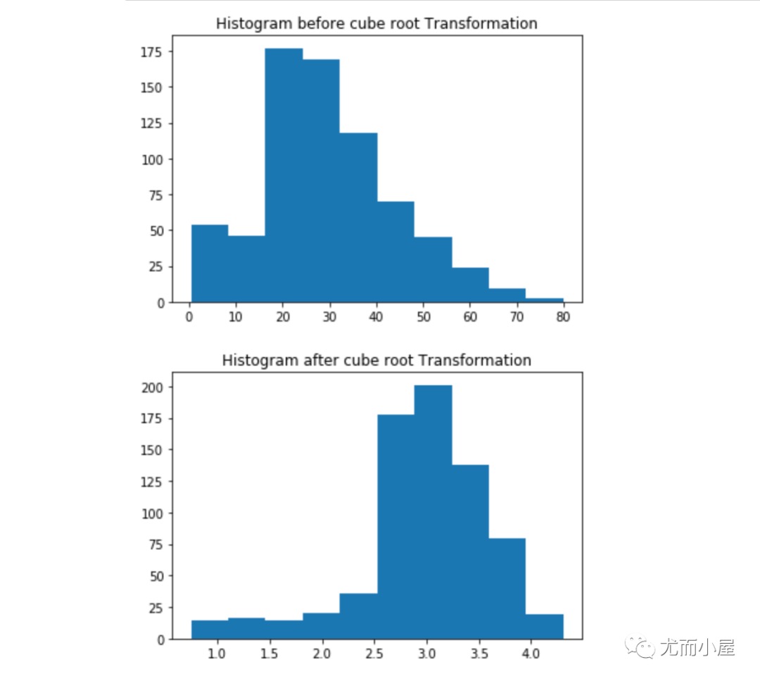
3. 立方根归一化：Cube Root Normalization
4. Box-Cox转换：Box-Cox transformation

# 尺度缩放

import pandas as pd
import numpy as np
import seaborn as sns
from matplotlib import pyplot as plt
from sklearn import preprocessing
train = pd.read_csv('cost-of-living-2018.csv')
plt.hist(train['Cost of Living Index'])
plt.title("Histogram before Scalling")
plt.show()   # 缩放前


scaler = preprocessing.StandardScaler()
train['Cost of Living Index'] = scaler.fit_transform(train['Cost of Living Index'].values.reshape(-1,1))
plt.hist(train['Cost of Living Index'])
plt.title("Histogram after Scalling")
plt.show()  # 缩放后

# 观察横坐标的值变化

# 2、基于对数变换

import pandas as pd
import numpy as np
import seaborn as sns
from matplotlib import pyplot as plt
train = pd.read_csv('cost-of-living-2018.csv')
sns.distplot(train['Cost of Living Index'])
plt.title("Distribution plot before Log transformation")
sns.despine()
plt.grid()
plt.show()

# ----变换后
train['Cost of Living Index'] = np.log(train['Cost of Living Index'])
sns.distplot(train['Cost of Living Index'])
plt.title("Distribution plot after Log transformation")
sns.despine()
plt.grid()
plt.show()

​

# 3、基于立方根转换

import pandas as pd
import numpy as np
import seaborn as sns
from matplotlib import pyplot as plt
train = pd.read_csv('Titanic.csv')
plt.hist(train['Age'])
plt.title("Histogram before cube root Transformation")
plt.show()

# 立方根变换
train['Age'] = (train['Age']**(1/3))
plt.hist(train['Age'])
plt.title("Histogram after cube root Transformation")
plt.show()

# 4、Box-Cox转换

import pandas as pd
import numpy as np
import seaborn as sns
from matplotlib import pyplot as plt
import scipy
train = pd.read_csv('cost-of-living-2018.csv')
sns.boxplot(train['Rent Index'])
plt.title("Box Plot before outlier removing")
plt.show()

train['Rent Index'],fitted_lambda= scipy.stats.boxcox(train['Rent Index'] ,lmbda=None)
sns.boxplot(train['Rent Index'])
plt.title("Box Plot after outlier removing")
plt.show()

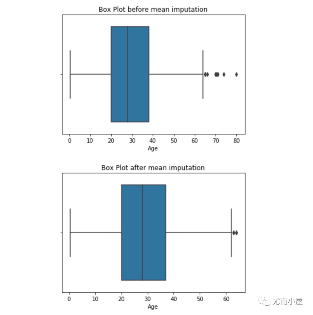
处理3：数值插补Imputation

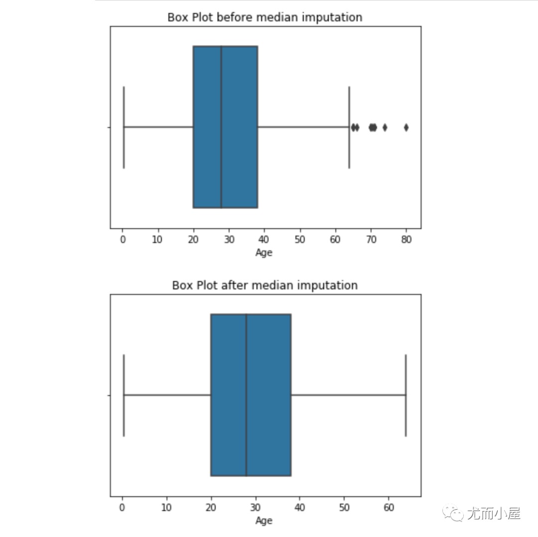
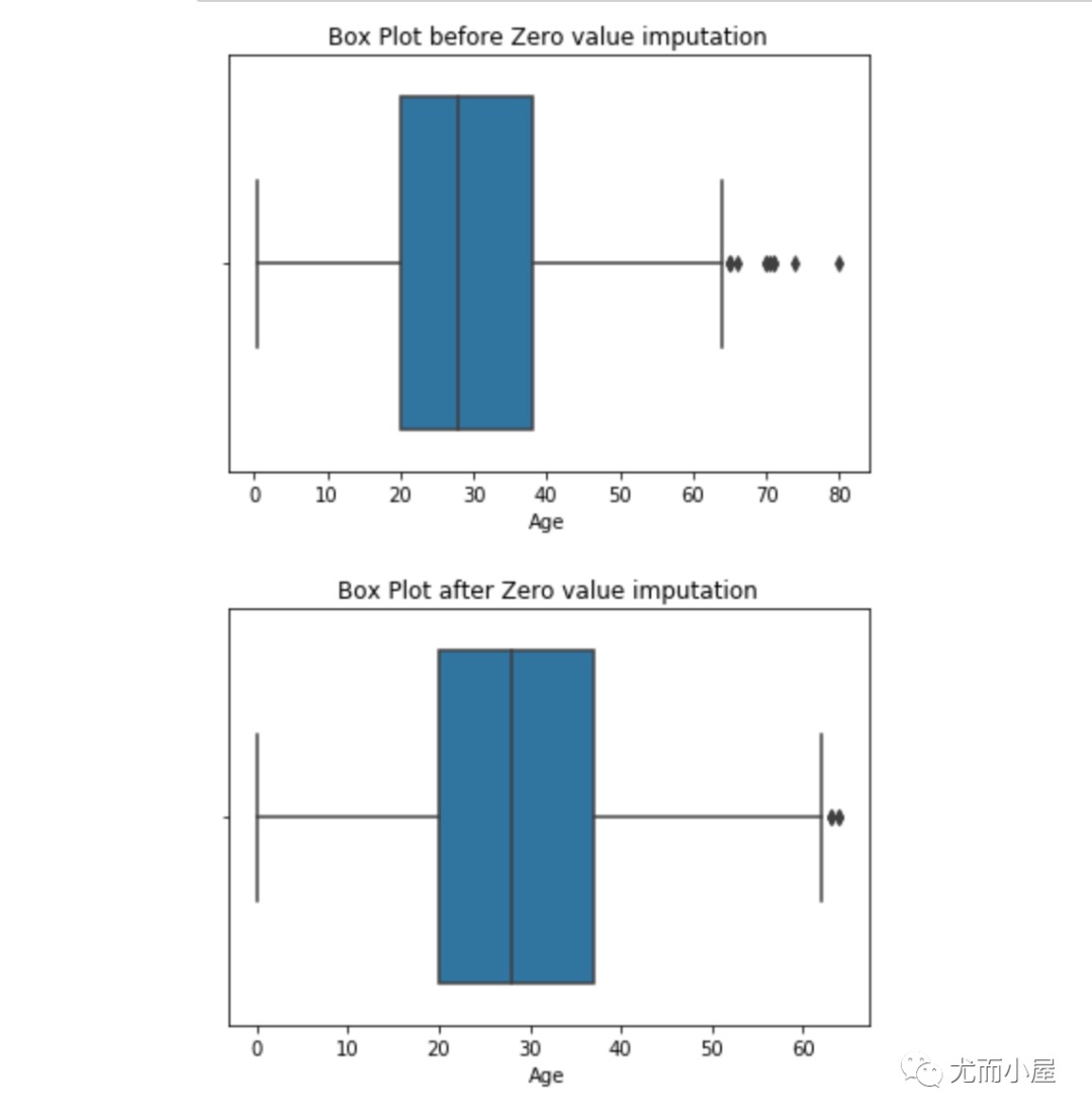
与缺失值的插补一样，我们也可以插补异常值。我们可以在此方法中使用均值、中值、零值。一般在这里使用中位数是最合适的，因为它不受异常值的影响。

# 基于均值插补

import pandas as pd
import numpy as np
train = pd.read_csv('Titanic.csv')
sns.boxplot(train['Age'])
plt.title("Box Plot before mean imputation")
plt.show()

q1 = train['Age'].quantile(0.25)
q3 = train['Age'].quantile(0.75)
iqr = q3-q1
Lower_tail = q1 - 1.5 * iqr
Upper_tail = q3 + 1.5 * iqr
m = np.mean(train['Age'])

for i in train['Age']:
    if i > Upper_tail or i < Lower_tail:
            train['Age'] = train['Age'].replace(i, m)  # 大于Upper或者小于Lower的值，用均值填充
sns.boxplot(train['Age'])
plt.title("Box Plot after mean imputation")
plt.show()

​
​

# 基于中位数插补

import pandas as pd
import numpy as np
train = pd.read_csv('Titanic.csv')
sns.boxplot(train['Age'])
plt.title("Box Plot before median imputation")
plt.show()

q1 = train['Age'].quantile(0.25)
q3 = train['Age'].quantile(0.75)
iqr = q3-q1
Lower_tail = q1 - 1.5 * iqr
Upper_tail = q3 + 1.5 * iqr
med = np.median(train['Age'])

for i in train['Age']:
    if i > Upper_tail or i < Lower_tail:
            train['Age'] = train['Age'].replace(i, med)
sns.boxplot(train['Age'])
plt.title("Box Plot after median imputation")
plt.show()

# 基于零值插补

import pandas as pd
import numpy as np
train = pd.read_csv('Titanic.csv')
sns.boxplot(train['Age'])
plt.title("Box Plot before Zero value imputation")
plt.show()

q1 = train['Age'].quantile(0.25)
q3 = train['Age'].quantile(0.75)
iqr = q3-q1
Lower_tail = q1 - 1.5 * iqr
Upper_tail = q3 + 1.5 * iqr

for i in train['Age']:
    if i > Upper_tail or i < Lower_tail:
            train['Age'] = train['Age'].replace(i, 0)
sns.boxplot(train['Age'])
plt.title("Box Plot after Zero value imputation")
plt.show()

处理4：离群点单独处理

如果存在大量的异常值并且数据集很小，在统计模型中我们应该将它们分开处理。一种方法是将离群点和非离群点视为两个不同的组，并为两个组构建单独的模型，然后组合输出。

总结

1. 当数据有异常值或偏斜时，中位数是数据集中趋势的最佳度量。
2. Winsorization Method 或 Percentile Capping 是其他方法中更好的异常值检测技术。
3. 中位数插补是最好的离群值插补方法。